Analysis of all Inderes recommendations

[vuh]

Mitä ja miksi?

Inderes on saavuttanut suurta suosiota suomalaisessa sijoittajayhteisössä. Inderesin mallisalkusta on tehty useita katsauksia ja jopa kvantitatiivinen analyysi yhteisön jäsenten toimesta (Inderes mallisalkku – kvantitatiivinen analyysi - Sijoittaminen - Inderes forum). Mallisalkku on voittanut vertailuindeksin poimimalla tarkkaan valitut voittajaosakkeet ja pitänyt niitä useita vuosia. Inderes seuraa nykyään kuitenkin reilusti yli sataa suomalaista pörssiyhtiötä: entäs kaikki suositukset joita Inderes on antanut?

Pyrin tässä analysoimaan kaikkien viimeaikaisten suositusten osuvuutta ja vastamaan näihin kysymyksiin:

• Kuinka monen yrityksen kohdalla suositukset ovat voittaneet `Indeksi’-strategian?
• Mikä olisi vuosituotto seuramaalla Inderesin suosituksia ja ` Indeksi’-strategiaa?
• Millä todennäköisyydellä tikkaa heittävä apina onnistuu yhtä hyvin, ts. tilastollinen merkittävyys?
• Mikä olisi strategioiden vuosituotto:
  • Yksittäisten osakkeiden kohdalla?
  • Yksittäisten analyytikoiden kohdalla?
  • Eri markkina-arvojen (large,mid,small, firstnorth) kohdalla?
• Mikä oli vuosituotto 2020-06-30 mennessä, ennen kuin mid/small cap yhtiöt raketoivat?

Tein tämän analyysin harrastuspohjalta, vaikka olenkin töissä koneoppimisen ja tilastotieteen parissa. Minulla ei ole taloudellisia siteitä Inderesiin ja olin ennen analyysiä skeptinen siitä kuinka hyvin suositukset ovat osuneet voittajaosakkeiden ulkopuolella. Analyysi osoitti kuitenkin jotain hyvin yllättävää…

Data on avointa ja julkaisen Python-koodit niin että laskelmat on mahdollista tarkistaa (GitHub - majuvi/suositukset)

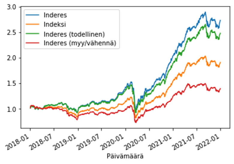
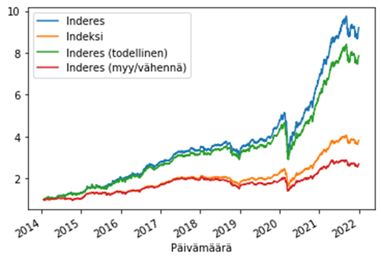
27.1.2022 Tämä on arvio suositusdataan perustuen. Lisätty postaus jossa on verrattu Inderes-salkkua ja Indeksi-salkkua kurssi- ja osinkohistoriadatasta muodostettuun tuottoindeksiin perustuen.

28.1.2022 Lisätty arvio sijoittajan todellisesta vuosituotosta ilman Inderes-efektiä tai mahdollista informaatioetua kun osaketta ostetaan vasta seuraavan päivän päätöskurssiin.

Data: suositukset

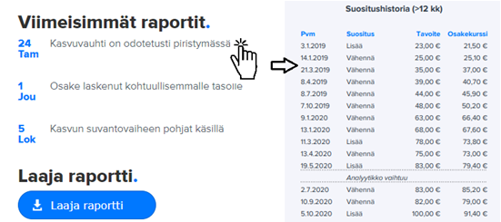
Inders julkaisee valitun pätkän suositushistoriaa raporttien yhteydessä, josta ne saa kätevästi kopioitua. Jotkut raportit vaativat Premium-jäsenyyden, mutta itse suositukset ovat julkisia. Keräsin viikonloppuna 22-23.1.2022 kaikista viimeisimmistä raporteista suositushistorian, ja liitin sen aiempaan historian jonka olin kerännyt kesällä 2020. Data sisältää tyypillisesti parista vuodesta muutaman vuoteen suositushistoriaa jokaisesta osakkeesta. Kerääminen vaatii hieman ahkeruutta tai itseäni enemmän osaamista webbiroboteista… Data prosessointi on minimaalista: SEK muuntaminen EUR suosituspäivänä, Suomisen englannin kääntämisen suomeksi, ja tusinan verran väärien päivämäärien korjaamista manuaalisesti.

Näistä raporteista saadaan tehtyä seuraavanlainen datajoukko:

Pvm,Suositus,Tavoite,Osakekurssi,Analyytikko,Osake
2019-04-09,Vähennä,8.5,8.87,Atte Riikola,Aallon Group
2019-08-23,Vähennä,9.0,9.5,Atte Riikola,Aallon Group
2019-09-30,Vähennä,9.0,9.34,Atte Riikola,Aallon Group
2019-12-12,Vähennä,9.9,10.45,Atte Riikola,Aallon Group
2020-02-14,Lisää,11.0,10.45,Atte Riikola,Aallon Group
…
2021-11-24,Vähennä,5.0,4.84,Olli Koponen,YIT

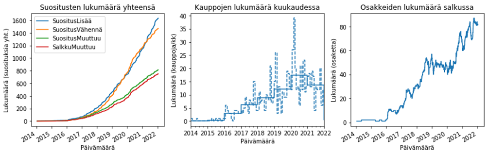
Yhteensä data sisältää 3109 riviä eli suositusta, 17 analyytikkoa, 139 osaketta.

Datassa on kaksi rajoitetta jotka on hyvä pitää mielessä 1) ‘Analyytiikko’ on viimeisin analytiikko, se ei ota huomioon jos analyytikko vaihtuu 2) Osakekurssi ei ota huomioon osinkoja, joten siitä laskettu tuotto on hieman pienempi kuin kokonaistuotto kurssimuutoksesta ja osingosta.

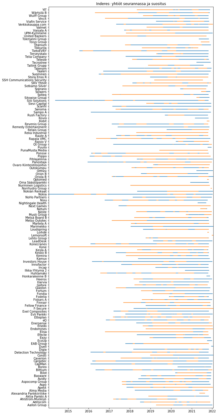
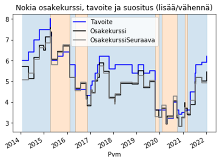
Tämä data voidaan kokonaisuudessa visualisoida esimerkiksi seuraavasti. Viivoissa väri esittää suositusta (sininen: Osta/Lisää ja oranssi: Myy/Vähennä) ja viivan pituus aikaa jolloin osake on Inderesin seurannassa. Graafista nähdään esimerkiksi, että Inderes on seurannut Siili Solutions osaketta useimmiten positiivisella suosituksella, ja Koneen osakketta myös useita vuosia ollen aina vähentämisen kannalla. Nokian osakkeen kohdalla suositus on vaihdellut enemmän. Oletan että “Inderes“-strategiaa seuraavan portfolio koostuu kunakin ajanhetkenä osakkeista, joilla on Lisää/Osta-suositus. “Buy/Hold“-strategiaa eli “Indeksiä” seuraavan portfolio olisi koostunut osakkeista jotka ovat Inderesin seurannassa riippumatta siitä onko suositus Lisää/Osta tai Myy/Vähennä. Valitettavasti tällä datalla ei voi täysin replikoida virallista indeksiä, koska data sisältää osakekurssin vain kun yhtiö on Inderesin seurannassa suosituksen antamisen hetkellä.

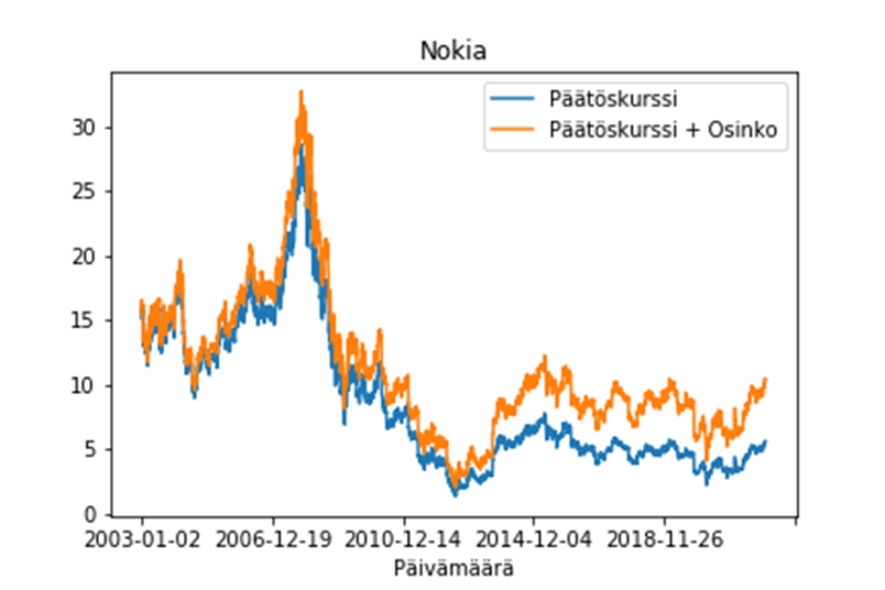
Esimerkki: Nokia

Selitän lyhyesti miten laskin vuosituoton. Käytän esimerkkinä Nokiaa:

Taulukkoon on nyt lisätty “Tuotto”, “Pitoaika” ja “Salkussa”. Nämä auttavat laskemaan tuoton kunkin suosituksen välillä ja määritellään seuraavasti:

• Tuotto: On osakkeen hinnanmuutokseen perustuva tuotto edellisestä suosituksesta nykyiseen suositukseen eli osakekurssi(t)/osakekurssi(t-1).
• Pitoaika: On päivien lukumäärä edellisestä suosituksesta nykyiseen suositukseen.
• Salkussa: Oliko osake Inderes-stragiaa seuraavan salkussa, eli oliko edellinen suositus Osta/Lisää.
  
  

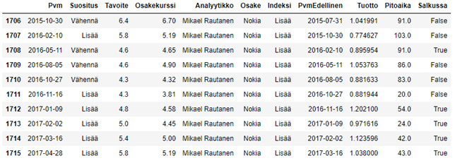
Esimerkissä Nokian tuotto on yksinkertaisesti näiden tuottojen tulo, eli 1.04 * 0.77 * …, mikä vastaa osakkeen viimeistä hintaa jaettuna ensimmäisellä hinnalla. Kokonaispitoaika päivinä on näiden pitoaikojen summa. Tuotto rippuu kuitenkin pitoajasta: keskimääräisen osakkeen tuotto on esim. 5% vuodessa, 10% kahdessa vuodessa, … jne. Siksi muutamme tuoton vuosituotoksi (CAGR) kaavalla: tuotto **(365/pitoaika).

Osta ja pidä

Tuotto         0.951049
Pitoaika    2911.000000
CAGR           0.993727

Eli nokia tuotti -5% hinnanmuutoksena seuranta-ajalla 2911 päivää, mikä vastaa noin -0.6% vuosituottoa.

Inderes-stragiaa seuraava omistaa osakkeen kun sillä on Osta/Lisää suositus. Tämän tuotto voidaan laskea ottamalla tuottojen tulo aikana jolloin osake on salkussa, ja kokonaispitoaika on näiden pitoaikojen summa. Jos haluaa ottaa huomioon Inderes-efektin ja mahdollisen pörssin sulkeutumisen jälkeisen informaation, täytyy käyttää seuraavan päivän osakekurssia. Kutsun tätä ”Todellinen” -tuotoksi. Tuotot eivät ole suoraan verrannollisia, koska osaketta pidetään vähemmän aikaa, mutta vuosituotoksi (CAGR) muutettuna näitä lukuja voidaan verrata:

Inderes

Tuotto         2.437720
Pitoaika    2097.000000
CAGR           1.167771

Inderes (Todellinen)

Tuotto         1.923152
Pitoaika    2097.000000
CAGR           1.120559

Eli Nokia tuotti 144% hinnanmuutoksena 2097 päivää positiivisella suosituksella, mikä tekee vuosituotoksi noin 17%. Jos ostetaan ja myydään vasta seuraavan päivän päätöskurssilla, saadaan vuosituotoksi 12%. Melkoinen analyysivelho tämä @Mikael_Rautanen !

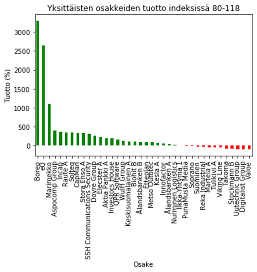
Kaikkien osakkeiden tuotto

Vastaava laskelma voidaan tehdä jokaiselle osakkeelle erikseen:

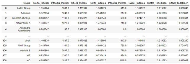
Miten monen osakkeen suositus voitti indeksin? Eli CAGR_Inderes > CAGR_Indeksi

True     99
False    40

99 osakkeen kohdalla suositukset voittivat indeksin ja 44 ei saavuttanut parempaa tuottoa kuin osta & pidä.

Miten monen osakkeen suositus voitti indeksin ilman Inderes-efektiä? Eli CAGR_Todellinen > CAGR_Indeksi

True     89
False    50

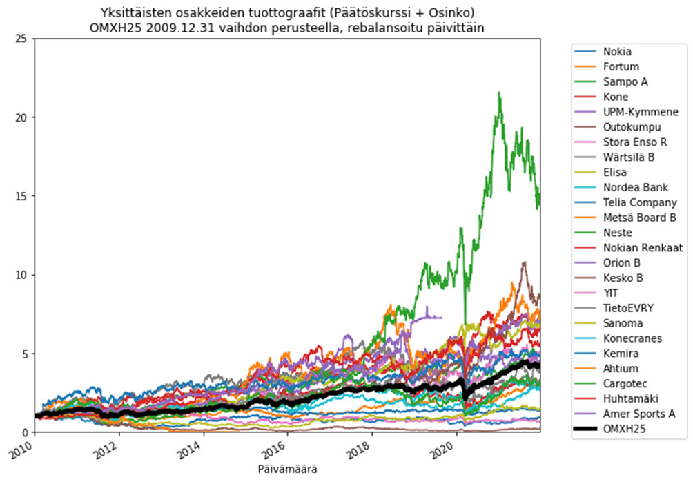
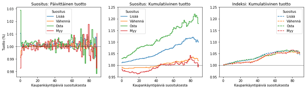
Alla visualisointi jossa verrataan jokaisen osakkeen Inderes-peesaajan ja osta&pidä-sijoittajan vuosituottoa:

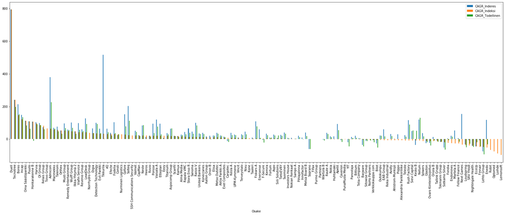
Joidenkin osakkeiden vuosituotto voi olla erittäin korkea, jos seuranta-aika ensimmäisestä suosituksesta viimeiseen suositukseen on erittäin lyhyt (esim. Duell) tai osakkeella on Lisää-suositus vain hyvin lyhyen aikaa. Esim kertaluonteinen 4% viikkotuotto osakkeella vastaisi koko vuodelle skaalattuna 1.04**(365/7)=7.73.. eli noin 673% vuosituottoa. Esimerkki myös havainnollistaa miksi vuosituottojen vertaaminen ei välttämättä vastaa kysymykseen miten sijoittaja voisi suoriutua. Tämä “vuosituotto” on mahdollista saada vain yhden viikon ajan vuodessa, eli tuotto on viikon aikana 4%, mutta muuten osakkeella olisi vähennä suositus jolloin siitä ei saisi tuottoja.

Portfolion tuotto

Tämän ottamiseksi huomioon tein seuraavan arviom portfolion vuosituosta:

1. Keskiarvo vuosituotoista: yksinkertainen lasku joka kuvaa Inderesin performanssia.
2. Vuosituotto sijoittamalla osakkeisiin joilla Lisää-suositus ja Inderesin seurannassa.

Näistä 2. kuvaa parhaiten todellisen sijoittajan suoriutumista. Aiemmassa viiva-kuvassa tämä vastaisi tilannetta jossa peesaaja katsoisi joka päivä inderesin seurannassa Lisää-suosituksella olevat osakkeet ja allokoisi portfolionsa tasaisesti näihin. Tämä on vähän monimutkaisempi lasku, siinä tuotto kunakin ajanhetkenä on portfolion osakkeiden tuottojen (r_i) aritmeettinen keskiarvo, joista otetaan ajanhetkien tuottojen geometrien keskiarvo, ottaen huomioon todennäköisyys että osake on portfoliossa (X_i). Laskin sen Monte Carlo-menetelmällä näytteistämällä portfolioita ajanhetkillä todennäköisyyksillä että osakkeet ovat seurannassa ja Lisää-suosituksella. Tämä vastaa portfolion keskimääräistä vuosituottoa ajan yli:

https://en.wikipedia.org/wiki/Product_integral ks. Law of large numbers

Saan seuraavat tuotot Inderes -sijoittajalle

1. 1.542
2. 1.386

Ja seuraavat tuotot Inderes (Todellinen)-sijoittajalle

1. 1.245
2. 1.251

Ja seuraavat tuotot Indeksi -sijoittajalle:

1. 1.181
2. 1.108

Keskimäärin siis Inderes-sijoittaja saa näiden muutaman vuoden aikana 38.6%-vuosituottoa osakkeiden hinnanmuutokseen perustuen, 25.1%-vuosituottoa jos otetaan huomioon Inderes-efekti käyttämällä seuraavan päivän päätöskurssia, missä Indeksi-sijoittaja jää 10.8% vuosituottoon. Raportoin myös näiden osakekohtaisten vuosituottojen (CAGR) yksinkertaisen keskiarvon koska se on helpompi ymmärtää: 54.2% Inderes vs. 24.5% Inderes (todellinen) vs. 18.1% Indeksi.

Ero on merkittävä mutta voiko se olla sattumaa? Tähän voidaan vastata seuraavalla tilastollisella testillä. Oletaan että Mikael Rautanen on palkannut lauman Apinoita heittämään tikkaa siitä annetaanko osakkeille Lisää- vai Vähennä-suositus. Simuloidaan tilannetta jossa Apinat antavat satunnaisesti kaikki suositukset, toistetaan tämä esimerkiksi 1000 kertaa, ja lasketaan apinoiden saama vuositotto:

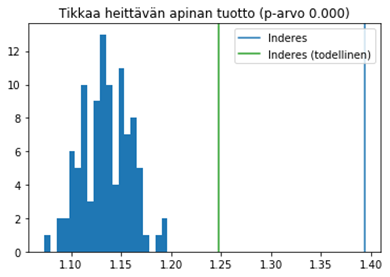
mean 1.133 sd 0.022 (12 sigmas Inderes, 5 sigmas Inderes (todellinen))

Havaitaan että 1000 simuloidusta Inderes-yhtiöstä jossa Apinat heittävät tikkaa yksikään ei pääse lähelle todellisen Inderesin vuosituottoa, vaan he saavat yleensä tuottoja väliltä 10-20%. Guruille selitys: permutaatiotesti jossa on nollahypoteesina “annetut suositukset on satunnaisesti allokoitu annettuihin ajanhetkiin”, p-arvo 0.000.

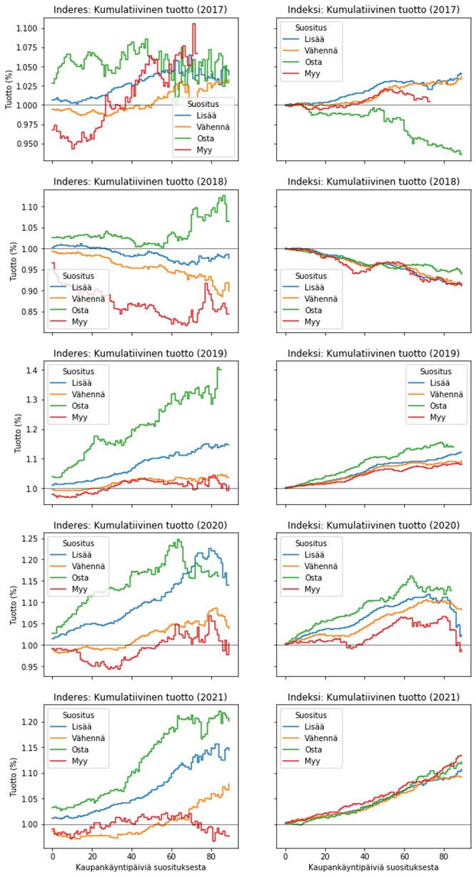
Portfolion tuotto: ennen “ränta pa ränta” -markkinaa

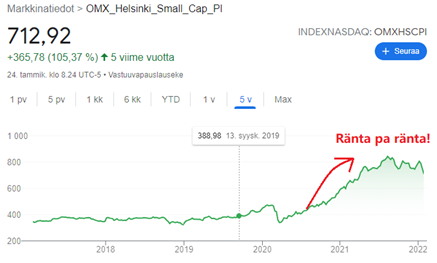
Nämä vuosituotot vaikuttavat liian hyvältä ollakseen totta, mutta ne selittyvät Helsingin pienyhtiöideksin 100% nousulla kesän 2020 jälkeen (Google: OMXHSCPI). Inderesin seuranta-aika yliedustaa tätä hetkeä. Tämän takia onkin mielenkiintoista varmistaa, että Inderesin menestys ei ole perustunut nykyiseen “ränta pa ränta”-markkinaan. Rajasin siksi datan päivämäärään 2020-06-30 ja tein samat laskut uudestaan.

Saan seuraavat tuotot Inderes-sijoittajalle

1. 1.432
2. 1.202

Ja seuraavat tuotot Inderes (Todellinen)-sijoittajalle

1. 1.129
2. 1.113

Ja seuraavat tuotot Indeksi-sijoittajalle:

1. 1.038
2. 0.971

Eli Inderesiä peesaava sijoittaja olisi saanut 20.2% vuosituoton hinnanmuutoksesta, 11.3% vuosituoton seuraavan päivän päätöskurssin hinnanmuutoksesta ja seurannasta koostettua indeksiä peesaava -3% vuosituottoa. Nämä ovat oletettavasti lähempänä tyypillistä tulevaisuuden markkinaa.

Vielä sama tikkaa heittävä Apina-simulaatio:

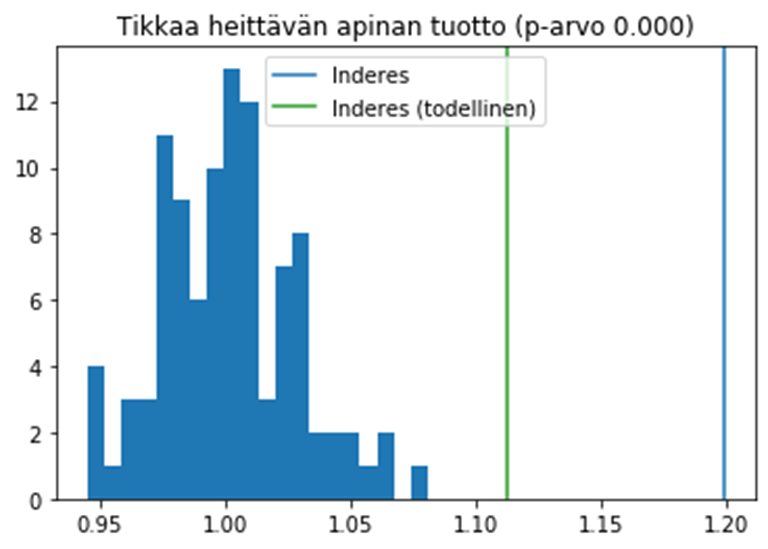
mean 1.002 sd 0.023 (7 sigmas Inderes, 4 sigmas Inderes (todellinen))

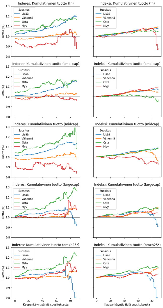
Markkina-arvot ja yksittäisten analyytikkojen suositukset

Käytössä on taas koko data. Voitaisiin argumentoida että Inderesin menestyminen perustuu vähän seurattuun pienyhtiö-kenttään, joten analysoin suositusten osuvuutta erikseen Helsingin pörssin suurimmille, keskisuurille, pienimmille ja First North-yhtiöille. Minulla ei ollut valitettavasti data suoraan markkina-arvoista, joten nämä perustuvat 1-40 eniten vaihdetuimpaan, 40-80 vaihdetuimpaan ja 81- 144 vähiten vaihdetuimpaan ajanhetkenä 31.12.2021. Omxh25* vastaa 1-25 eniten vaihdettua.

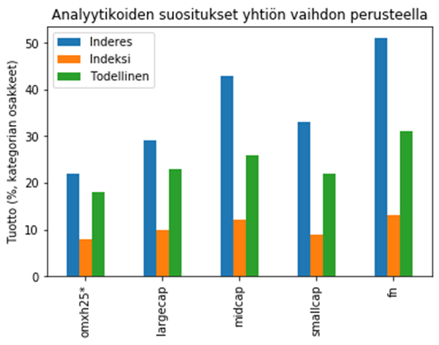
Vaikuttaa että pienemmissä yhtiöissä on helpompi tehdä ylituottoa, mutta ylituottoa Inderes on saanut kaikkien kategorioiden osakkeilla.

Seuraavassa kuvaajassa laskin minkälaisen tuoton yksittäistä analyytikkoa peesaava sijoittaja olisi saanut (lasku 3.) ja vertasin tätä indeksiin joka kostuu tämän analyytikon seuraamista yhtiöistä. Siinä ei ole otettu huomioon analyytikon vaihtumista, joten ei sovi suoraan kyseisen analyytikon mittariksi:

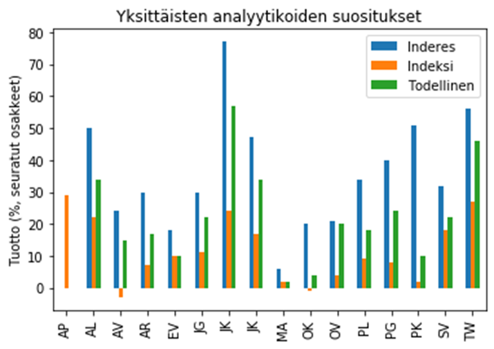
Huomataan että lähes kaikki Indersin analyytikot voittivat oman vertailuindeksinsä, eli tulokset eivät selity yksittäisillä huippunimillä. Kaikki ovat tähtianalyytikkoja!

Lopuksi

Inderesin keskimääräinen 38.6%-vuosituotto suositusdatasta laskettuna vrt. Inderesin todellinen vuosituotto 25.1% seuraavan kaupankäyntipäivän päätöskurssilla vs. osta&pidä 10.8%-vuosituotto osakkeiden hintojen muutokseen perustuen on uskomaton saavutus. Ennen ”ränta pa ränta” kesää 2020 saavutettu Inderesin 20.2% vuosituotto ja 11.3% todellinen vuosituotto on erittäin kunnioitettava indeksin -3% rinnalla. Inderes-efekti tai pörssin sulkeutumisen jälkeen julkaistu informaatio vaikuttaa yllättävän paljon todellisen sijoittajan saamaan performanssiin, mutta ero indeksiin on tästä huolimatta merkittävä. Tämä oli nopea viikonloppuna tehty harjoitus, ja laskut on vielä hyvä tarkistaa. Kysymykset, asiallinen kritiikki ja ehdotukset analyysin laajentamiseksi ovat tervetulleita.

[no1z]

Interesting analysis, and nice to see that pandas comes naturally to you

I recall that @Kelpieracer had done a similar analysis some time ago; in addition to the code, data can probably also be found here:

GitHub - Kelpieracer/analysts-recommendations-strategy

[Tottero]

All I can say is, hats off. Both to the analyst and to Inderes.

[Onni_Maiha]

Great research and strong results! I’m wondering if Inderes’ figures include some undeserved information advantage. For example, a situation where a company issues a positive announcement after the stock market closes, and then Inderes updates its analysis from “reduce” to “add” before the start of the next trading day. However, the share price in the analysis is based on the closing price of the previous trading day, which gives Inderes’ analysis an information advantage relative to that price. A similar situation can occur when an update following a negative announcement turns from “add” to “reduce.”

[Kelpieracer]

Good job, and it’s great to see you’ve got a knack for this!

I couldn’t be bothered to copy-paste all the companies I was following back in the day, so it’s good that’s been done now. And my own results have been confirmed.

Did you analyze the different recommendations separately? I concluded that the “add” recommendation was a bit useless, and there was no difference from the “reduce” recommendation. Following only the “buy” recommendation yielded excess returns.

And indeed, the Inderes effect eats into returns. So, buys and sells need to be looked at from the close of the next trading day.

I didn’t check where you got the price data; I just used Yahoo and adjclose (which accounts for dividends and splits), but one has to be careful with data errors.

Edit: Let’s save the old ones here

Inderesin kahvihuone (Osa 2)

Inderesin kahvihuone (Osa 2)

And a disclaimer

Inderesin kahvihuone (Osa 2)

[vuh]

It’s great to hear that someone else has done similar analysis. I tried searching the forum but missed these posts. I’d love to hear more about this, perhaps in this thread, if you have more results. I haven’t specifically studied Buy/Add or Sell/Reduce recommendations, but I assumed both correspond to adding or removing a stock from a portfolio. Good idea to test this!

The good thing about this recommendation dataset is that it doesn’t require separate price data because the current stock price is given along with the recommendation. As a couple of commenters pointed out, its downside is that it cannot be corrected for information appearing after the market closes and the Inderes effect, as this would require the next day’s closing price. In addition, the formula is an estimate of the average annual return. The idea is to add this when I have time.

[KalleH]

@Kelpieracer

And indeed, the Inderes effect eats away at returns. So, buys and sells must be viewed from the close of the next trading day.

Wouldn’t the next day’s opening price be best?

[Kelpieracer]

Or their average…
So, Yahoo provides AdjClose directly, not AdjOpen, though it can be easily calculated.
In any case, I think it’s more accurate to use the adjusted figure since it includes splits and dividends.
Edit. I have a personal problem called a “day job,” and I usually don’t have time to trade before evening, which is why I might be fixated on the closing price.

[Kelpieracer]

@vuh

It’s great to hear that someone else has done a similar analysis. I tried searching the forum, but I missed these posts.

Actually, when I was writing it, I already thought they would get lost in the lounge… good that you made your own thread.

@vuh

would require the closing price of the next day.

Yeah, you can easily get the price history from that yahoo_fin library once you’ve got pandas (Pandas) under control.

@vuh

It would be great to hear more about this in this thread, if you have more results.

I’ve simulated all sorts of things, but I don’t recall anything more specifically related to Inderes recommendations.
Sector, size, and continent rotation strategies with ETFs (I get returns compared to B&H, but lose to MSCI World), and trading with Nordnet Markets products on equity and metal targets, that’s what I did last.
Inderes recommendations (and model portfolio) have had the best backtests. With Nordnet Markets products, you can make returns by quant trading stocks, but it takes a huge amount of your own and machine time. I’ve written about some of these in the algorithms thread.

[vuh]

This morning, I added the actual return received by an investor, where the Inderes investor’s buys and sells are made at the closing price of the next day. I need to investigate the Yahoo API. Currently, I downloaded the price history from Kauppalehti’s (Finnish financial newspaper) website, which I understand is also adjusted for splits, etc.:

Edit: Added to the first post, many thanks to @Sijoittaja-alokas and @Yu_Gong

[Kelpieracer]

Great and useful work, @vuh!

Edit. Is it possible to find out from that data how the Inderes effect has developed over the years? I.e., when was this advantage eaten away?

[vuh]

A quick new analysis first thing in the morning. I’ve now calculated the return of a balanced index of all shares and compared it to an index compiled from Inderes’ recommendations. That is, an index investor owns all shares on the Helsinki Stock Exchange and First North in equal euro amounts, and an Inderes investor owns all shares with Inderes’ buy/add recommendations in equal euro amounts. Both indices are rebalanced daily in the calculations. I performed balancing and daily rebalancing because it is easiest with this data.

First, it is necessary to retrieve the price and dividend history and calculate the total return for each share. For this purpose, I fetched the closing prices and dividends for trading days starting from 01-01-2000 and ending on 31-12-2021. The idea is to assume that on the ex-dividend date (when a buyer of the share no longer receives the dividend), the dividend is reinvested by buying the same share with the same amount of money as received from the dividend. The purchase is made at that day’s closing price. Consequently, if the dividend is d and the price is P, the investor has d/P new shares in the company. As a result, the number of shares increases by (1+d/P) each time the company pays a dividend. The total return is then each day’s closing price multiplied by the investor’s total number of shares. Below is an example of Nokia, where the total return from time T to time T+K is simply Total Return (T+K) / Total Return (T) (orange line). In the long run, dividends have a significant impact:

By taking the total return of all shares, various indices and nice graphs can be calculated. Neste performed strongly, but Ahtium (ex Talvivaara) took a quick nosedive:

It is important to remember here that small companies have performed significantly better during the period, so the balanced index I used yields better returns than the official OMXHGI index:

This is often explained by a few super successful companies (Boreo, eQ, Marimekko):

Inderes vs. Return Index

Now to the results. If we look at the previous graph visualizing the data set in the first post, we observe that in 2014, only a couple of companies were being tracked: Nokia (fluctuating), Siili Solutions (add). Because of this, the outperformance of the ‘index’ formed from 2014 onwards would be mainly based on Siili’s positive recommendation. Therefore, I will initially show a more representative index formed from 2018-01-01 onwards.

From 2018 onwards

In the following index, “Inderes” buys a share into the portfolio on the same day an Add/Buy recommendation is given, and sells the share when a Reduce/Sell recommendation is given. “Inderes (actual)” is corrected for potential informational advantage and the Inderes effect by buying the share only at the closing price of the next trading day. The investor’s portfolio thus consists of all companies for which Inderes has an Add or Buy recommendation. The “Index” tracks all companies on the Helsinki Stock Exchange and First North on an equal-weighted basis. “Inderes (reduce)” is the “Inderes” recommendations in reverse.

I get the following annual portfolio returns by 31-12-2021:

Inderes                  1.285636
Index                  1.175273
Inderes (actual)     1.254914
Inderes (sell/reduce)    1.086588

And the following by 2020-06-30 before the “räntä pa räntä” (slushy snow) summer.

Inderes                  1.127808
Index                  1.040166
Inderes (actual)     1.100969
Inderes (sell/reduce)    0.983676

From 2014 onwards

This calculation might be misleading due to the small number of shares on which the recommendations were based, but I will include it anyway.

I get the following annual portfolio returns by 31-12-2021:

Inderes                  1.322538
Index                  1.183842
Inderes (actual)     1.296388
Inderes (sell/reduce)    1.132848

And the following by 2020-06-30 before the “räntä pa räntä” summer.

Inderes                  1.265387
Index                  1.131018
Inderes (actual)     1.241634
Inderes (sell/reduce)    1.100633

Conclusions

The actual annual return of the Inderes portfolio between 01-01-2018 and 31-12-2021 (4 years), when most stocks were under coverage, was 25.5% per year, while the annual return of the balanced index consisting of all stocks remained at 17.5%. The OMXHGI index yielded an annual return of ~13% during the period, which is significantly less (no FN, market cap weighted). The return between 01-01-2018 and 2020-06-30, before the “räntä pa räntä” summer, was 10.1% for the Inderes portfolio and 4.0% for the balanced index of all stocks.

In a previous post, we estimated the annual return of the Inderes (actual) portfolio to be 24.8% and the annual return of the index price change to be 10.7%. Before summer 2020, we estimated the annual return of the Inderes (actual) portfolio to be 11.3% and the annual return of the index price change to be -3%. The return based on the actual index is very close to previous estimates for Inderes, but the index’s return improved by approximately +7%. This should be explained by taking into account dividends and companies not under coverage (or no longer under coverage). However, Inderes still clearly beats the index

[Fyys]

Have you considered a calculation exercise that also accounts for taxes and trading fees? On the OST (Osakesäästötili - Share Savings Account) side, you can, of course, trade tax-free, but in that case, the portfolio size is probably such that trading fees per trade are significant. At least assuming such a high level of diversification. For example, how much does the return decrease when 0.3-1% in fees is taken from each trade?

[vuh]

Interesting question, I could do it. Nordnet’s pricing would charge an Inderes-active investor 0.10%-0.15% in fees if they could invest about €4667-€5000 at once, and one could still consider subtracting the bid/ask spread from that. If one does it daily, there won’t be any returns

It also occurred to me about the ‘Inderes (Actual)’ index that while it measures a private investor’s return well, in principle it is unfair when measuring Inderes’s performance because they could have bought the stock before the Inderes effect, insofar as this effect is based on other investors’ excitement and not on information after the close of trading.

Added: Trading Costs

I started calculating trading costs and tax effects, but it’s much more complicated than I thought. If there’s no cash in the portfolio, a selling strategy should be made when Inderes gives an ‘Add’ recommendation; for example, selling the best-performing stock by halving the position, etc. Whether to hold cash and with what lump sum to trade. To avoid trading costs, it might be more reasonable to invest a larger sum in a stock at once than to maximize diversification, and then one would have to randomly choose where to invest. What about rebalancing, etc.? Then one would also have to subtract tax from dividends and capital gains tax at the time of sale.

However, I made you @Fyys this simple ‘small investor’s Stock Savings Account’ calculation on a napkin . Below is the number of positive and negative recommendations over time, the number of recommendation changes over time, and the number of portfolio trades over time. The latter is slightly smaller because starting monitoring with a negative recommendation does not change the portfolio. We see that an Inderes investor following recommendations would make 4-40 trades per month, averaging 14 trades. Nordnet’s pricing Tier 2 (11-50 trades/month) is 0.10% / min €5. Add and reduce recommendations come equally often, and nowadays Inderes follows most companies, so we could simplify that the portfolio would now have 80 stocks, and these are changed according to recommendations.

This would mean investing €50,000/80 = €625 in one stock, a fee per trade of €5/€625 = 0.8%, and an annual fee of 14 * 12 * €5/€50,000 = 1.68%. If €1,000,000 were available, €12,500 would be invested in one stock, a fee per trade of 0.1%, and an annual fee of 0.21%. 14 * 12 = 168 trades are made during the year, meaning the turnover is 2.1x the portfolio, hence the fee is 2 times. This 1.68% fee gradually decreases to this 0.21% minimal fee when the portfolio value exceeds 80 * (€5/0.1%) = €400,000.

Earlier, I estimated that Inderes (actual) has generated an outperformance of 6-8% compared to the OMXH&FN balanced and daily rebalanced, completely cost-free hypothetical return index. If we subtract this 0.21% - 1.68% fee, depending on the portfolio size from €400,000 to €50,000, we are still in profit

[vuh]

The Inderes Effect

By popular demand (@Kelpieracer), I spent an evening conducting another analysis of the Inderes effect, which is the phenomenon where a stock’s price jumps immediately when Inderes issues a Buy/Accumulate recommendation and falls with a Sell/Reduce recommendation. Many have surely noticed this phenomenon in the stock market, so here is data on the average Inderes effect. I analyzed it by:

• Recommendation type: Buy/Accumulate/Reduce/Sell
• Market capitalization: fn/small cap/medium cap/large cap/OMXH25
• Year: 2017-2021

The idea is to measure how much a stock yields after Inderes issues a recommendation. Let’s define 0 as the recommendation date, 1 as the next day, 2 as the day after that, and so on. For comparison, I also calculated the average return of all other stocks, i.e., the ‘index’ for each recommendation from the recommendation date onwards. We could assume that the recommendation correlates strongly with the stock’s performance but not with the index, unless ‘accumulate’/‘reduce’ recommendations are generally given more when the market as a whole is trending up/down.

Buy/Accumulate/Reduce/Sell

The following image visualizes the average daily percentage return based on the type of recommendation, and the average cumulative return of an individual stock and the index over the subsequent trading days. It is observed that on the day of the recommendation, a ‘Buy’ recommendation immediately yields +3%, an ‘Accumulate’ recommendation +1%, a ‘Reduce’ recommendation slightly less than -1%, and a ‘Sell’ recommendation slightly less than -2% return. The effect continues, albeit more subdued, for the next couple of days. It’s interesting to note that the effect does not reverse over time; that is, the stock does not return to its starting level. Cumulatively, it is observed that the return difference of ‘Buy’/‘Accumulate’ stocks compared to the index increases over time, meaning the outperformance is not solely due to the Inderes effect, although it is significant. The return of ‘Reduce’/‘Sell’ stocks rises slightly above 0% after a couple of months, which is a significant underperformance compared to the index.

fn/small cap/medium cap/large cap/omxh25

Let’s examine cumulative returns based on turnover on 2021-12-31, where I categorized stocks into different classifications: fn (First North) / small cap (81-144 least traded) / med cap (41-80 traded) / large cap (1-40 most traded) / omxh25* (1-25 most traded). It is observed that the Inderes effect is largest in small and medium-sized companies, on average even +/- 5% for ‘Buy’/‘Sell’ recommendations. In large companies, a small positive +1% effect can be observed for ‘Buy’/‘Accumulate’ recommendations, but no negative effect. Inderes’ outperformance can be observed in all categories. This does not appear to be based on market timing as stocks with positive recommendations only catch up to the corresponding index.

2017-2021

Finally, the same analysis for different years. I don’t see a clear trend that the Inderes effect has increased or decreased, but it’s interesting to observe how recommendations work in both falling (2018) and rising (2021) markets. During the COVID-19 pandemic (2020), Inderes also seemed to succeed in market timing because the index also yielded differently based on the type of recommendation. That is, ‘Reduce’ recommendations correlated with a general decline in stocks, and ‘Accumulate’ recommendations correlated with a general rise in stocks. Inderes’ strength, however, lies in stock picking, as the best returns were made by picking winners in a generally rising market (2019, 2020, 2021).

[Ripelein]

Portfolio management is indeed a difficult topic, and there are many different options. In my own project, the problem has become clearly apparent recently, as the investment options have increased while the sum to be invested has remained the same. The intention is to invest more in better targets than in less good ones, while still ensuring sufficient diversification.

For example, with a minimum trade of €4,000 within a €100,000 portfolio, and a maximum investment of €20,000 in a single company. In this case, it is possible to invest clearly different amounts in five investment targets. If the number of investment targets grows to 15, the maximum available for one company is only €6,666. At this point, clear differences in investment amounts can no longer be made. One must choose an amount between €4,000 and €6,666, and no additional investments can be made.

With cheaper brokers, transaction costs can be reduced. If the choices are good, even an increase in the relative share of costs is not necessarily a bad thing. A third option could be to prune poorer investments, for example, to eight, which would allow investing a maximum of €12,500 in a single company. If the investment decision is guided by Buy/Sell information, pruning is quite difficult quantitatively.

When investing a fixed sum, one is also exposed to fluctuations in the number of investment targets. If anyone has information about good literature concerning portfolio management, please share.

[Alfons_Knautmauer]

Just throwing this out as an idea (since there’s been some interesting discussion about target prices): what kind of returns would one get by investing directly based on Inderes’ target prices?

The portfolio would be allocated so that Target Price - Current Price (I believe this is the potential in Inderes’ stock comparison table) would correspond to the stock’s weight in the portfolio.

This could be done long-only, considering only positive potentials. Or “market-neutrally,” so that negative potentials would be shorted proportionally.

If someone has some free time, interest, and their existing Python scripts could be adapted without major changes, it would be interesting to see. And it would provide an interesting backdrop to the discussion caused by the fluctuation of the risk-free rate.

[vuh]

There’s a lot to be found in academic literature, but the answer is complex and context-dependent . However, I do remember that many studies have found that 1/N balancing works surprisingly well in reality. Here are a couple of strong papers:

The modern portfolio theory pioneered by Markowitz (1952) is widely used in practice and extensively taught to MBAs. However, the estimated Markowitz portfolio rule and most of its extensions not only underperform the naive 1/ N rule (that invests equally across N assets) in simulations, but also lose money on a risk-adjusted basis in many real data sets.
https://www.sciencedirect.com/science/article/abs/pii/S0304405X10001893

Of the 14 models we evaluate across seven empirical datasets, none is consistently better than the 1/ N rule in terms of Sharpe ratio, certainty-equivalent return, or turnover, which indicates that, out of sample, the gain from optimal diversification is more than offset by estimation error. https://academic.oup.com/rfs/article-abstract/22/5/1915/1592901?login=false

This even refers to the book Rationality for Mortals: How People Cope with Uncertainty, stating that Markowitz, the developer of Modern Portfolio Theory, would have used this rule himself: Heuristics and Robustness in Asset Allocation: The 1/N Rule, “Hard” Constraints and Fractional Kelly Strategies | macroresilience

It would require an expert on the topic and months of time to summarize these formulas and wisdoms. However, by browsing the sources, I get the impression that this simple strategy can be surprisingly close to optimal: for example, 80 stocks at €5000 each, and a stock is sold if Inderes gives a Reduce recommendation, and a stock with an Increase recommendation that is not yet in the portfolio is bought in its place.

[Mikael_Rautanen]

Wow! Thanks for the analysis

If there’s any data you’d otherwise have to extract from reports, feel free to contact us and we can see if that data can be easily found in the database as a single package. We’ve already provided historical data for some theses and master’s theses.

[greenhornet]

I was just about to ask if the recommendation data was available, @vuh? The data wasn’t visible on GitHub.